Sharpe Ratio Trading: A Practical Guide for Traders

Sharpe Ratio Trading: A Practical Guide for Traders
The Sharpe ratio measures how much return you earn per unit of risk taken, calculated as excess return divided by the standard deviation of those returns. For traders, it answers one question that matters above all others: is this strategy actually earning its risk, or just getting lucky with volatility?

Here’s what that means in practice. A strategy returning 20% annually sounds great until you learn it swings 40% in either direction. A strategy with similar returns but much lower volatility is a far better business. The Sharpe ratio captures that distinction in a single number, making it the standard tool for comparing strategies, sizing positions, and spotting when a live strategy starts to degrade.
Quick benchmarks to orient yourself:
- S&P 500 long-term Sharpe sits in the 0.4–0.6 range, your baseline for any active strategy
- Retail traders generally target a Sharpe ratio in the 1.0–2.0 range as a realistic benchmark for good risk-adjusted performance.
- Quantitative research desks often require 2.0 or higher before a strategy enters serious development
This guide covers the exact formula and notation, step-by-step calculation in Python and Excel, professional thresholds, the ratio’s real limitations, and backtest hygiene rules that prevent inflated numbers from misleading you.
Table of Contents
- What is the Sharpe ratio and how does it work for trading?
- How do you calculate Sharpe ratio from your trading returns?
- What counts as a good Sharpe ratio for traders?
- When does the Sharpe ratio break down?
- Worked examples: seeing the numbers in action
- Backtest hygiene: using Sharpe correctly in research pipelines
- Your Sharpe ratio checklist before comparing or scaling strategies
- How Optiqtrades surfaces risk-adjusted metrics for options traders
- Key Takeaways
- The metric is only as honest as the data behind it
- See your risk-adjusted metrics on Optiqtrades
- Useful sources for further study
What is the Sharpe ratio and how does it work for trading?
The Sharpe ratio, introduced by William F. Sharpe in 1966 under the name “reward-to-variability ratio,” is defined as:
S = (Rp − Rf) ÷ σp
Where Rp is the portfolio or strategy return, Rf is the risk-free rate, and σp is the standard deviation of excess returns. The result is unitless, which is what makes it useful for comparing strategies across different asset classes, frequencies, and sizes.
Ex-post vs. ex-ante Sharpe
Traders use two versions. The ex-post (realized) Sharpe is computed from historical returns and tells you how a strategy actually performed. The ex-ante (expected) Sharpe is forward-looking, built from forecasted returns and estimated volatility, and is used when allocating capital across strategies before live deployment. Most of the time, when traders say “Sharpe ratio,” they mean ex-post.
Choosing the right risk-free rate
For U.S.-based trading, the standard choice is the 3-month Treasury bill yield. Match the rate to your return period: if you’re computing daily returns, divide the annualized T-bill yield by 252. For weekly returns, divide by 52. For market-neutral strategies that are fully hedged and carry no directional exposure, some practitioners use zero as the risk-free rate, since the strategy has no opportunity cost relative to holding cash.
- Use the 3-month T-bill for most equity and options strategies
- Use the federal funds rate as an alternative for very short-term strategies
- Use zero for genuinely market-neutral, dollar-neutral books.
Pro Tip: Period-matching matters more than the exact rate. A 5% annual T-bill divided by 252 is about 0.0198% per day. Forgetting to scale it down inflates your excess return and produces a Sharpe that looks better than it is.
How do you calculate Sharpe ratio from your trading returns?
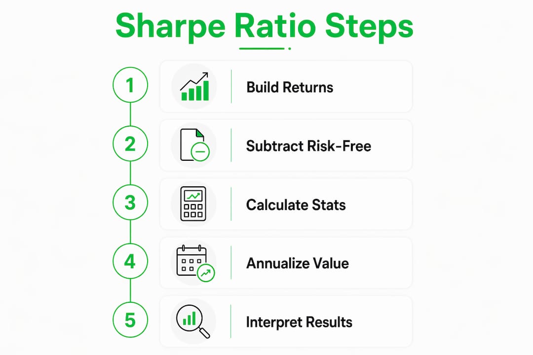
The calculation has four steps. Follow them in order and you’ll avoid the most common mistakes.
Step 1: Build your periodic returns series
Start with your P&L or price series and convert it to percentage returns for each period. For a daily series, that’s (Price_t / Price_{t-1}) − 1. For a trade-by-trade P&L, use net P&L divided by starting capital for each period. Avoid mixing trade-level returns with time-period returns in the same series.
For small samples, be cautious. Fewer than roughly 30 observations produces a noisy estimate that can mislead you in either direction.
Step 2: Subtract the matching-period risk-free rate
Daily excess return = Daily return − (Annual T-bill yield ÷ 252). For a 5% annual T-bill, that’s approximately 0.0198% per day. This step is small in magnitude but correct in principle.
Step 3: Compute mean and standard deviation of excess returns
import pandas as pd
import numpy as np

# Assume 'returns' is a pandas Series of daily net returns (decimal)
rf_daily = 0.05 / 252  # 5% annual T-bill scaled to daily

excess_returns = returns - rf_daily
mean_excess = excess_returns.mean()
std_excess = excess_returns.std(ddof=1)  # sample std dev

period_sharpe = mean_excess / std_excess
annualized_sharpe = period_sharpe * np.sqrt(252)
print(f"Annualized Sharpe: {annualized_sharpe:.4f}")
In Excel, the equivalent formula for a daily returns column in A2:A253 is:
=AVERAGE(A2:A253-rf_daily)/STDEV(A2:A253-rf_daily)*SQRT(252)
Step 4: Annualize using the √N rule
The annualized Sharpe is √N × (mean excess return ÷ std dev), where N is the number of trading periods per year. Use 252 for daily equity returns, 52 for weekly, 12 for monthly. For intraday strategies, N is the number of trading periods per year based on your actual trade frequency, not 24 × 252.
Pro Tip: Autocorrelation in daily returns (common in trend-following strategies) inflates the annualized Sharpe. If your daily returns are serially correlated, use a Newey-West correction or compute Sharpe on weekly returns and scale by √52 instead.
What counts as a good Sharpe ratio for traders?
The honest answer: it depends on your strategy type and trading frequency. Here are the thresholds practitioners actually use.
| Strategy Type | Sharpe Range | Notes |
|---|---|---|
| S&P 500 buy-and-hold | 0.4–0.6 | Long-term historical baseline |
| Retail discretionary | 0.5–1.0 | Acceptable; below 0.5 is poor |
| Active retail target | 1.0–2.0 | Good; worth allocating to |
| Quant research minimum | 2.0+ | Institutional threshold for development |
| High-frequency strategies | 3.0–10.0+ | Frequent wins compress volatility |
| Suspicious backtest | >3.0 (retail) | Often signals overfitting |

Warren Buffett’s Berkshire Hathaway produced a Sharpe of approximately 0.76 over a multi-decade period, higher than any other stock or mutual fund with a comparable history. That number should recalibrate expectations: you do not need a Sharpe of 3.0 to build serious wealth.
Why frequency changes everything. High-frequency strategies naturally compress return volatility because they generate many small, consistent wins. A market-making algorithm running thousands of trades per day can show a Sharpe in the single digits or higher without any overfitting. A monthly swing trader with a Sharpe of 1.5 is doing extremely well by comparison. Always compare Sharpe values across strategies with similar frequencies.
Statistical callout: A Sharpe estimated from three months of daily returns has a standard error large enough to make a “true” Sharpe of 1.0 look anywhere from 0.4 to 1.6. Short samples are not just imprecise; they are actively misleading. Aim for at least one full year of returns before drawing conclusions.
When does the Sharpe ratio break down?
The Sharpe ratio rests on assumptions that trading returns routinely violate. Knowing where it fails is as important as knowing how to calculate it.
Core failure modes:
- Non-normal returns: Fat tails and skewness mean standard deviation understates real risk. A strategy selling out-of-the-money puts can show a high Sharpe for years, then suffer a single catastrophic loss that the ratio never predicted.
- Upside penalization: Sharpe treats a big winning month the same as a big losing month. Both increase standard deviation and lower the ratio. For options strategies with positive skew, this produces a misleadingly low number.
- Autocorrelation: Serially correlated returns (common in trend-following) inflate the annualized Sharpe by making volatility appear lower than it is.
- Short samples: As noted above, fewer observations mean wider confidence intervals around the estimate.
Alternatives and when to use them
Sortino ratio replaces the denominator with downside deviation only, ignoring positive returns. For options strategies or any payoff with meaningful positive skew, Sortino presents a more investor-relevant view because it stops penalizing you for winning big. Use it when your return distribution is visibly right-skewed.
Information ratio measures excess return over a benchmark divided by tracking error. Use it when your strategy is explicitly benchmark-relative, such as a long/short equity book targeting alpha over the S&P 500.
Calmar ratio divides annualized return by maximum drawdown. Use it when drawdown tolerance is the binding constraint, which is common for managed accounts and prop desks with hard stop-loss rules.
For options strategies with volatile market conditions, pairing Sharpe with Sortino and Calmar gives a far more complete picture than any single metric alone.
Pro Tip: If Sharpe and Sortino rank your strategies in the same order, stop debating which ratio to use. Research across thousands of funds confirms the rankings are highly correlated. Focus on robustness and execution risk instead.
Worked examples: seeing the numbers in action
Example 1: Daily returns for a discretionary day trader
Assume 252 trading days, mean daily excess return of 0.08%, standard deviation of daily excess returns of 0.55%.
| Metric | Value |
|---|---|
| Mean daily excess return | 0.08% |
| Std dev of daily excess returns | 0.55% |
| Period (daily) Sharpe | 0.145 |
| Annualized Sharpe (× √252) | a value indicating strong risk-adjusted performance |
That annualized Sharpe of 2.31 puts this strategy solidly in the “excellent” retail range, as retail targets for a good risk-adjusted strategy are typically in the 1.0–2.0 range. But notice how the daily Sharpe of 0.145 looks tiny in isolation. Always annualize before comparing across strategies.
Example 2: Market-neutral strategy
A dollar-neutral long/short book with no net market exposure. Risk-free rate subtraction is set to zero (no opportunity cost relative to cash). Mean daily return: 0.04%, std dev: 0.30%.
- Period Sharpe = 0.04 / 0.30 = 0.133
- Annualized = 0.133 × √252 = a value indicating strong risk-adjusted performance
A Sharpe ratio of 2.0 or higher with no directional beta is genuinely attractive to institutional allocators.
Example 3: Options strategy with asymmetric payoff
A covered-call writing strategy earns steady small credits but occasionally gives back gains in a strong rally. Mean monthly excess return: 1.2%, std dev: 3.8% (inflated by a few large upside months).
- Period Sharpe = 1.2 / 3.8 = 0.316
- Annualized = 0.316 × √12 = a value indicating moderate risk-adjusted return (Sharpe)
- Downside deviation (monthly): 1.9%
- Sortino = 1.2 / 1.9 = 0.632 → annualized = 2.19
The Sortino is twice the Sharpe because the volatility driving the denominator is mostly upside. For tracking options trades systematically, recording both metrics side by side reveals this distortion immediately.
Backtest hygiene: using Sharpe correctly in research pipelines
A high backtest Sharpe is not evidence of a good strategy. It is a hypothesis that requires validation.
Required adjustments before trusting a backtest Sharpe
- Include transaction costs and slippage. Many high-Sharpe backtests collapse once realistic costs are applied. Use per-share or per-contract commissions plus a conservative slippage estimate based on average spread.
- Add borrow and financing costs for leveraged or short positions. Ignoring these inflates net returns and therefore inflates Sharpe.
- Eliminate lookahead bias. Any use of future data in signal construction will produce a Sharpe that is impossible to replicate live.
- Check for data-snooping. If you tested 50 parameter combinations and picked the best, your Sharpe is biased upward. Apply a Bonferroni correction or use a deflated Sharpe ratio framework.
- Run out-of-sample validation. Reserve at least 20–30% of your data as a holdout set. A strategy that maintains its Sharpe out-of-sample is far more credible than one that only shines in-sample.
- Use rolling windows. Compute Sharpe over rolling 6-month or 12-month windows. Consistent Sharpe across regimes is a stronger signal than a high average over the full period.
Sampling guidance. For day traders, use at least one full quarter of returns, ideally a calendar year. For monthly-frequency strategies, three years of data is a reasonable minimum. Always report trade count and max drawdown alongside Sharpe so readers can assess whether the sample is meaningful.
Pro Tip: Bootstrap resampling is one of the most practical stress tests available. Resample your returns with replacement 1,000 times and compute the Sharpe distribution. If the 5th percentile of that distribution is still above your threshold, you have a more credible strategy than a single-point estimate can confirm.
Your Sharpe ratio checklist before comparing or scaling strategies
Run through this before using any Sharpe number to make a capital allocation decision.
- Confirm return frequency. Daily, weekly, or monthly? Use the matching N for annualization.
- Verify the return series is net of costs. Gross returns produce a flattering but useless Sharpe.
- Subtract the period-matched risk-free rate. Scale the T-bill yield to your return frequency.
- Check sample size. Fewer than 30–60 observations? Flag the estimate as preliminary.
- Annualize correctly. Multiply the period Sharpe by √N, not N.
- Compare with Sortino and Calmar. If they tell a different story, investigate why before proceeding.
- Pull max drawdown. A Sharpe of 1.5 with a 40% max drawdown is a different risk profile than one with a 10% drawdown.
- Check for autocorrelation. Run a Ljung-Box test on your excess returns if you suspect serial correlation.
Pro Tip: If your backtest Sharpe is above 3.0 and you’re a retail trader, treat it as an indication of possible overfitting or data issues. Recheck your cost assumptions, look for lookahead bias, and run the strategy on a fresh data window before trusting the number.
How Optiqtrades surfaces risk-adjusted metrics for options traders
Optiqtrades is built around the idea that performance data should be transparent and comparable, not buried in a spreadsheet only the strategy creator can read. The platform’s leaderboard surfaces trader performance ranked by risk-adjusted metrics, so you can see who is generating returns efficiently rather than just who had the biggest month.
The AI Options Strategist evaluates every trade in real time, giving you an AI-powered read on risk and reward before you copy a position. That evaluation layer is what separates a community platform from a simple copy-trade feed.
How to apply the Sharpe workflow on Optiqtrades:
- Browse the trader directory and filter by win rate, returns, and follower count to identify candidates worth deeper analysis
- Review a trader’s return history and drawdown profile alongside their Sharpe to confirm consistency
- Use the AI Strategist evaluation to check whether the underlying options positions carry asymmetric risk that Sharpe alone might understate. When evaluating traders on the platform, look for moderate Sharpe ratios in the 1.0–2.0 range paired with low max drawdown and a meaningful trade count.
- Follow traders whose metrics hold up across multiple market regimes, not just recent momentum
Pro Tip: When evaluating traders on the platform, look for moderate Sharpe (roughly 1.0–2.0) paired with low max drawdown and a meaningful trade count. An outlier Sharpe from 10 trades tells you almost nothing.
Key Takeaways
The Sharpe ratio is the most practical single metric for comparing trading strategies on a risk-adjusted basis, but it requires correct calculation, sufficient sample size, and pairing with drawdown and alternative metrics to avoid misleading conclusions.
| Point | Details |
|---|---|
| Core formula | Sharpe = (strategy return − risk-free rate) ÷ standard deviation of excess returns, annualized by multiplying by √N. |
| Realistic benchmarks | S&P 500 baseline is 0.4–0.6; retail target is 1.0–2.0; quant research minimum is typically 2.0 or higher. |
| Calculation discipline | Always use net-of-cost returns, period-matched risk-free rate, and at least one year of data before trusting the estimate. |
| Key limitation | Sharpe penalizes upside and downside volatility equally; pair it with Sortino for skewed payoffs and Calmar for drawdown-sensitive mandates. |
| Optiqtrades application | Optiqtrades leaderboards and AI evaluations surface risk-adjusted trader metrics so you can compare and copy strategies with more than just raw returns. |
The metric is only as honest as the data behind it
The most common misuse of the Sharpe ratio in live trading is treating it as a verdict rather than a signal. Traders compute a Sharpe of 1.8 from three months of returns and start scaling up, when the honest interpretation is: “this looks promising, now I need six more months to know if it’s real.”
The other pattern worth naming: chasing a high Sharpe by over-optimizing parameters. A strategy tuned to produce a Sharpe of 2.5 in-sample that drops to 0.6 out-of-sample is not a 2.5 Sharpe strategy. It’s a 0.6 Sharpe strategy with a flattering backtest. Consistency across time periods and market regimes is worth more than a peak number from a favorable window.
Treat Sharpe the way a good operator treats any business KPI: a moderate, stable number with a clear explanation is more valuable than an impressive number you can’t reproduce. The traders who build durable track records are rarely the ones with the highest Sharpe in any given quarter. They’re the ones whose Sharpe doesn’t collapse when conditions change.
See your risk-adjusted metrics on Optiqtrades
Calculating Sharpe manually is a good skill. Having it computed, displayed, and ranked across hundreds of real traders is better.
Optiqtrades gives options traders a free community platform where leaderboards rank traders by performance metrics, not just raw returns. The AI Options Strategist evaluates every trade in real time, and the copy-trade feature lets you mirror positions from traders whose risk-adjusted track record you’ve verified. You can browse trader profiles, check drawdown history, and follow strategies that match your risk tolerance, all without a subscription to get started.
Visit Optiqtrades to browse the leaderboard, review trader metrics, and start applying the Sharpe framework to real, live performance data. Platform metrics are based on user-reported and brokerage-connected data; always verify independently before copying any trade.
Useful sources for further study
- Sharpe Ratio for Algorithmic Trading | QuantStart — the most practical technical treatment of annualization, frequency effects, and backtest hygiene for algo traders
- The Sharpe Ratio (original paper) | Stanford / William F. Sharpe — the primary source; worth reading for the ex-ante vs. ex-post distinction and the zero-investment strategy framework
- Sharpe vs. Sortino: Does It Matter? | CAIA — empirical analysis across 2,000+ funds showing the two ratios produce nearly identical rankings in most cases
- Sharpe Ratio | Investopedia — clear explanation of the Sortino difference and when downside deviation is the better denominator
- Sharpe Ratio: 6 Things You Need to Know | TradingSim — retail-focused benchmarks, sample-size guidance, and overfitting warnings in plain language
- Understanding the Sharpe Ratio | BullTraders — practical threshold ranges and the case for treating moderate, stable Sharpe as more valuable than an outlier number
- Buffett’s Alpha (Digest Summary) | CFA Institute — the empirical estimate of Berkshire’s Sharpe ratio, useful for calibrating expectations against a real-world benchmark
Next step: Run your own Sharpe calculation using the Python snippet above, then cross-check it against the trader metrics on the Optiqtrades platform to see how your strategy compares to the community.